# hide
# based on EnergyStorage_I_ANNO-2.ipynb

#no 1-hot encoding for the decision variable
#use the buy-low-sell-high PFA policyIn Part 2 we used 1-hot encoding for the decision variable. We also optimized a Bellman policy - one in the Value Function Approximation (VFA) class. This policy was be based on Bellman’s exact dynamic programming approach making use of Backward Dynamic Programming (BDP).
In Part 3 (and Part 4) we change the 1-hot encoding of the decision variable to something more scalable. We will have a single decision variable (\(x_{t,GB}\)) where a positive value indicates the amount bought, a negative value the amount sold, and a zero value when neither happened. The \(GB\) stands for ‘Grid-to-Battery’. When the flow is from grid to battery, \(x_{t,GB}\) will have a positive value. When the flow is reversed, i.e. battery to grid, \(x_{t,GB}\) will have a negative value. In the future, the number of decision variables will be increased as needed. Eventually we will have the decision vector:
\((x_{t,EL}, x_{t,EB}, x_{t,GL}, x_{t,GB}, x_{t,BL})\)
In Part 3 we explore again the buy-low-sell-high policy.
0 STRUCTURE & FRAMEWORK
The overall structure of this project and report follows the traditional CRISP-DM format. However, instead of the CRISP-DM’S “4 Modeling” section, we inserted the “6 step modeling process” of Dr. Warren Powell in section 4 of this document.
The example explored (but also modified) in this report comes from Dr. Warren Powell (formerly at Princeton). It was chosen as a template to create a POC for a client. It was important to understand this example thoroughly before embarking on creating the POC. Dr Powell’s unified framework shows great promise for unifying the formalisms of at least a dozen different fields. Using his framework enables easier access to thinking patterns in these other fields that might be beneficial and informative to the sequential decision problem at hand. Traditionally, this kind of problem would be approached from the reinforcement learning perspective. However, using Dr. Powell’s wider and more comprehensive perspective almost certainly provides additional value.
Here is information on Dr. Powell’s perspective on Sequential Decision Analytics.
The original code for this example can be found here.
In order to make a strong mapping between the code in this notebook and the mathematics in the unified framework, many variable names in the original code have been adapted. Here is a summary of the mapping between the mathematics and the variable names in the code:
- Superscripts
- variable names have a double underscore to indicate a superscript
- \(X^{\pi}\): has code
X__pi, is read X pi
- Subscripts
- variable names have a single underscore to indicate a subscript
- \(S_t\): has code
S_t, is read ‘S at t’ - \(M^{Spend}_t\) has code
M__Spend_twhich is read: “MSpend at t”
- Arguments
- collection variable names may have argument information added
- \(X^{\pi}(S_t)\): has code
X__piIS_tI, is read ‘X pi in S at t’ - the surrounding
I’s are used to imitate the parentheses around the argument
- Next time/iteration
- variable names that indicate one step in the future are quite common
- \(R_{t+1}\): has code
R_tt1, is read ‘R at t+1’ - \(R^{n+1}\): has code
R__nt1, is read ‘R at n+1’
- Rewards
- State-independent terminal reward and cumulative reward
- \(F\): has code
Ffor terminal reward - \(\sum_{n}F\): has code
cumFfor cumulative reward
- \(F\): has code
- State-dependent terminal reward and cumulative reward
- \(C\): has code
Cfor terminal reward - \(\sum_{t}C\): has code
cumCfor cumulative reward
- \(C\): has code
- State-independent terminal reward and cumulative reward
- Vectors where components use different names
- \(S_t(R_t, p_t)\): has code
S_t.R_tandS_t.p_t, is read ‘S at t in R at t, and, S at t in p at t’ - the code implementation is by means of a named tuple
self.State = namedtuple('State', SNames)for the ‘class’ of the vectorself.S_tfor the ‘instance’ of the vector
- \(S_t(R_t, p_t)\): has code
- Vectors where components reuse names
- \(x_t(x_{t,GB}, x_{t,BL})\): has code
x_t.x_t_GBandx_t.x_t_BL, is read ‘x at t in x at t for GB, and, x at t in x at t for BL’ - the code implementation is by means of a named tuple
self.Decision = namedtuple('Decision', xNames)for the ‘class’ of the vectorself.x_tfor the ‘instance’ of the vector
- \(x_t(x_{t,GB}, x_{t,BL})\): has code
- Use of mixed-case variable names
- to reduce confusion, sometimes the use of mixed-case variable names are preferred (even though it is not a best practice in the Python community), reserving the use of underscores and double underscores for math-related variables
1 BUSINESS UNDERSTANDING
The following business description comes from the free book by Dr. Powell, Sequential Decision Analytics and Modeling:
New Jersey is looking to develop 3,500 megawatts (MW) of offshore wind generating power. A challenge is that wind (and especially offshore wind) can be highly variable, due in part to the property that wind power (over intermediate ranges) increases with the cube of wind speed. This variability is depicted in figure 9.1, developed from a study of offshore wind. Energy from wind power has become popular in regions where wind is high, such as the midwestern United States, coastal regions off of Europe, the northeast of Brazil, and northern regions of China (to name just a few). Sometimes communities (and companies) have invested in renewables (wind or solar) to help reduce their carbon footprint and minimize their dependence on the grid. It is quite rare, however, that these projects allow a community to eliminate the grid from their portfolio. Common practice is to let the renewable source (wind or solar) sell directly to the grid, while a company may purchase from the grid. This can be useful as a hedge since the company will make a lot of money during price spikes (prices may jump from $20 per megawatt-hour (MWh) to $300 per MWh or more) that offsets the cost of purchasing power during those periods.
A challenge with renewables is handling the variability. While one solution is to simply pump any energy from a renewable source into the grid and use the tremendous power of the grid to handle this variability, there has been considerable interest in using storage (in particular, battery storage) to smooth out the peaks and valleys. In addition to handling the variability in the renewable source, there has also been interest in using batteries to take advantage of price spikes, buying power when it is cheap (prices can even go negative) and selling it back when they are high. Exploiting the variability in power prices on the grid is known as battery arbitrage.
This problem will provide insights into virtually any inventory/storage problem, including - Holding cash in mutual funds A bank has to determine how much of its investment capital to hold in cash to meet requests for redemptions, versus investing the money in loans, stocks and bonds. - Retailers (including both online as well as bricksandmortar stores) have to manage inventories of the hundreds of thousands of products. - Auto dealers have to decide how many cars to hold to meet customer demand. - Consulting firms have to decide how many employees to keep on staff to meet the variable demand of different consulting projects.
Energy storage is a particularly rich form of inventory problem.
2 DATA UNDERSTANDING
Next, we will start to look at the data that is provided for this problem.
#hide
from google.colab import drive
drive.mount('/content/gdrive', force_remount=True)
root_dir = "/content/gdrive/My Drive"
base_dir = root_dir + '/Powell/EnergyStorage_I'
Mounted at /content/gdrive# import pdb
from collections import namedtuple, defaultdict
import numpy as np
import pandas as pd
import matplotlib.pyplot as plt
from copy import copy
import time
from scipy.ndimage.interpolation import shift
import pickle
from bisect import bisect
import math
from pprint import pprint
import matplotlib as mpl
pd.options.display.float_format = '{:,.4f}'.format
pd.set_option('display.max_columns', None)
pd.set_option('display.max_rows', None)
pd.set_option('display.max_colwidth', None)
! python --version
# 3.8.10; found it changed on 3/10/23Python 3.9.16DeprecationWarning: Please use `shift` from the `scipy.ndimage` namespace, the `scipy.ndimage.interpolation` namespace is deprecated.
from scipy.ndimage.interpolation import shiftdef process_raw_price_data(file, params):
DISC_TYPE = "FROM_CUM"
#DISC_TYPE = "OTHER"
print("Processing raw price data. Constructing price change list and cdf using {}".format(DISC_TYPE))
tS = time.time()
# load energy price data from the Excel spreadsheet
raw_data = pd.read_excel(file, sheet_name="Raw Data")
# look at data spanning a week
data_selection = raw_data.iloc[0:params['T'], 0:5]
# rename columns to remove spaces (otherwise we can't access them)
cols = data_selection.columns
cols = cols.map(lambda x: x.replace(' ', '_') if isinstance(x, str) else x)
data_selection.columns = cols
# sort prices in ascending order
sort_by_price = data_selection.sort_values('PJM_RT_LMP')
#print(sort_by_price.head())
hist_price = np.array(data_selection['PJM_RT_LMP'].tolist())
#print(hist_price[0])
max_price = pd.DataFrame.max(sort_by_price['PJM_RT_LMP'])
min_price = pd.DataFrame.min(sort_by_price['PJM_RT_LMP'])
print("Min price {:.2f} and Max price {:.2f}".format(min_price,max_price))
# sort prices in ascending order
sort_by_price = data_selection.sort_values('PJM_RT_LMP')
# calculate change in price and sort values of change in price in ascending order
data_selection['Price_Shift'] = data_selection.PJM_RT_LMP.shift(1)
data_selection['Price_Change'] = data_selection['PJM_RT_LMP'] - data_selection['Price_Shift']
sort_price_change = data_selection.sort_values('Price_Change')
# discretize change in price and obtain f(p) for each price change
max_price_change = pd.DataFrame.max(sort_price_change['Price_Change'])
min_price_change = pd.DataFrame.min(sort_price_change['Price_Change'])
print("Min price change {:.2f} and Max price change {:.2f}".format(min_price_change,max_price_change))
# there are 191 values for price change
price_changes_sorted = sort_price_change['Price_Change'].tolist()
# remove the last NaN value
price_changes_sorted.pop()
if DISC_TYPE == "FROM_CUM":
# discretize price change by interpolating from cumulative distribution
xp = price_changes_sorted
fp = np.arange(len(price_changes_sorted) - 1) / (len(price_changes_sorted) - 1)
cum_fn = np.append(fp, 1)
# obtain 30 discrete prices
discrete_price_change_cdf = np.linspace(0, 1, params['nPriceChangeInc'])
discrete_price_change_list = []
for i in discrete_price_change_cdf:
interpolated_point = np.interp(i, cum_fn, xp)
discrete_price_change_list.append(interpolated_point)
else:
price_change_range = max_price_change - min_price_change
price_change_increment = price_change_range / params['nPriceChangeInc']
discrete_price_change = np.arange(min_price_change, max_price_change, price_change_increment)
discrete_price_change_list = list(np.append(discrete_price_change, max_price_change))
f_p = np.arange(len(price_changes_sorted) - 1) / (len(price_changes_sorted) - 1)
cum_fn = np.append(f_p, 1)
discrete_price_change_cdf = []
for c in discrete_price_change_list:
interpolated_point = np.interp(c, price_changes_sorted, cum_fn)
discrete_price_change_cdf.append(interpolated_point)
price_changes_sorted = np.array(price_changes_sorted)
discrete_price_change_list = np.array(discrete_price_change_list)
discrete_price_change_cdf = np.array(discrete_price_change_cdf)
discrete_price_change_pdf = discrete_price_change_cdf - shift(discrete_price_change_cdf,1,cval=0)
mean_price_change = np.dot(discrete_price_change_list,discrete_price_change_pdf)
#print("discrete_price_change_list ", discrete_price_change_list)
#print("discrete_price_change_cdf", discrete_price_change_cdf)
#print("discrete_price_change_pdf", discrete_price_change_pdf)
print("Finishing processing raw price data in {:.2f} secs. Expected price change is {:.2f}. Hist_price len is {}".format(time.time()-tS,mean_price_change,len(hist_price)))
#input("enter any key to continue...")
exog_params = {
"hist_price": hist_price,
"price_changes_sorted": price_changes_sorted,
"discrete_price_change_list": discrete_price_change_list,
"discrete_price_change_cdf": discrete_price_change_cdf}
return exog_paramsseed = 189654913
file = 'Parameters.xlsx'# NOTE:
# R__max: unit is MWh which is an energy unit
# R_0: unit is MWh which is an energy unit
parDf = pd.read_excel(f'{base_dir}/{file}', sheet_name='ParamsModel', index_col=0); print(f'{parDf}')
# parDict = parDf.set_index('Index').T.to_dict('list')#.
parDict = parDf.T.to_dict('list') #.
params = {key:v for key, value in parDict.items() for v in value}
params['seed'] = seed
params['T'] = min(params['T'], 192); print(f'{params=}') 0
Index
Algorithm BackwardDP
T 195
eta 0.9000
R__max 1
R_0 1
params={'Algorithm': 'BackwardDP', 'T': 192, 'eta': 0.9, 'R__max': 1, 'R_0': 1, 'seed': 189654913}parDf = pd.read_excel(f'{base_dir}/{file}', sheet_name='GridSearch', index_col=0); print(parDf)
# parDict = parDf.set_index('Index').T.to_dict('list')#.
parDict = parDf.T.to_dict('list')
paramsPolicy = {key:v for key, value in parDict.items() for v in value}; print(f'{paramsPolicy=}')
params.update(paramsPolicy); pprint(f'{params=}') 0
Index
theta_sell_min 10
theta_sell_max 100
theta_buy_min 10
theta_buy_max 100
theta_inc 1
paramsPolicy={'theta_sell_min': 10, 'theta_sell_max': 100, 'theta_buy_min': 10, 'theta_buy_max': 100, 'theta_inc': 1}
("params={'Algorithm': 'BackwardDP', 'T': 192, 'eta': 0.9, 'R__max': 1, 'R_0': "
"1, 'seed': 189654913, 'theta_sell_min': 10, 'theta_sell_max': 100, "
"'theta_buy_min': 10, 'theta_buy_max': 100, 'theta_inc': 1}")parDf = pd.read_excel(f'{base_dir}/{file}', sheet_name='BackwardDP', index_col=0); print(parDf)
# parDict = parDf.set_index('Index').T.to_dict('list')#.
parDict = parDf.T.to_dict('list')
paramsPolicy = {key:v for key, value in parDict.items() for v in value}; print(f'{paramsPolicy=}')
params.update(paramsPolicy); pprint(f'{params=}') 0
Index
nPriceChangeInc 50
priceDiscSet 1, 0.5
run3D False
paramsPolicy={'nPriceChangeInc': 50, 'priceDiscSet': '1, 0.5', 'run3D': False}
("params={'Algorithm': 'BackwardDP', 'T': 192, 'eta': 0.9, 'R__max': 1, 'R_0': "
"1, 'seed': 189654913, 'theta_sell_min': 10, 'theta_sell_max': 100, "
"'theta_buy_min': 10, 'theta_buy_max': 100, 'theta_inc': 1, "
"'nPriceChangeInc': 50, 'priceDiscSet': '1, 0.5', 'run3D': False}")if isinstance(params['priceDiscSet'], str):
price_disc_list = params['priceDiscSet'].split(",")
price_disc_list = [float(e) for e in price_disc_list]
else:
price_disc_list = [float(params['priceDiscSet'])]
params['price_disc_list'] = price_disc_list; print(f'{price_disc_list=}')price_disc_list=[1.0, 0.5]pprint(f"{params=}")
#input("enter any key to continue...")("params={'Algorithm': 'BackwardDP', 'T': 192, 'eta': 0.9, 'R__max': 1, 'R_0': "
"1, 'seed': 189654913, 'theta_sell_min': 10, 'theta_sell_max': 100, "
"'theta_buy_min': 10, 'theta_buy_max': 100, 'theta_inc': 1, "
"'nPriceChangeInc': 50, 'priceDiscSet': '1, 0.5', 'run3D': False, "
"'price_disc_list': [1.0, 0.5]}")#exog_params is a dictionary with three lists:
# hist_price, price_changes_list, discrete_price_change_cdf
# exog_params = process_raw_price_data(f'{base_dir}/{file}', params)
exogParams = process_raw_price_data(f'{base_dir}/{file}', params) #.
# print(f"{exogParams['hist_price']=}")
# print(f"{exogParams['price_changes_sorted']=}")
# print(f"{exogParams['discrete_price_change_list']=}")
# print(f"{exogParams['discrete_price_change_cdf']=}")Processing raw price data. Constructing price change list and cdf using FROM_CUM
Min price 0.00 and Max price 107.34
Min price change -54.40 and Max price change 65.81
Finishing processing raw price data in 3.46 secs. Expected price change is 1.28. Hist_price len is 192print("Ingesting raw price data for understanding.")
# load energy price data from the Excel spreadsheet
raw_data = pd.read_excel(f'{base_dir}/{file}', sheet_name="Raw Data")
# look at data spanning a week
df_raw = raw_data.iloc[0:params['T'], 0:5]
# rename columns to remove spaces (otherwise we can't access them)
cols = df_raw.columns
cols = cols.map(lambda x: x.replace(' ', '_') if isinstance(x, str) else x)
df_raw.columns = cols
df_raw.head()Ingesting raw price data for understanding.| Time | Day | Hour | PJM_DA_LMP | PJM_RT_LMP | |
|---|---|---|---|---|---|
| 0 | 1.0000 | 2005-01-01 00:00:00 | 1.0000 | 25.7200 | 18.9100 |
| 1 | 2.0000 | 2005-01-01 01:00:00 | 2.0000 | 23.0800 | 14.2700 |
| 2 | 3.0000 | 2005-01-01 02:00:00 | 3.0000 | 21.0000 | 9.6700 |
| 3 | 4.0000 | 2005-01-01 03:00:00 | 4.0000 | 20.0000 | 17.6800 |
| 4 | 5.0000 | 2005-01-01 04:00:00 | 5.0000 | 20.0400 | 11.8800 |
from certifi.core import where
def plot_data(df):
  n_charts = 2
  ylabelsize = 16
  fig, axs = plt.subplots(n_charts, sharex=True)
  fig.set_figwidth(10); fig.set_figheight(7)
  fig.suptitle('PRICE OF ELECTRICITY [$/MWh]', fontsize=20)
  i = 0
  axs[i].set_ylim(auto=True); axs[i].spines['top'].set_visible(False); axs[i].spines['right'].set_visible(True); axs[i].spines['bottom'].set_visible(True)
  axs[i].plot(df['PJM_DA_LMP'], 'r')
  axs[i].set_ylabel('$\mathrm{PJM\ DA\ LMP}$', rotation=0, ha='right', va='center', fontweight='bold', size=ylabelsize);
  i = 1
  axs[i].set_ylim(auto=True); axs[i].spines['top'].set_visible(False); axs[i].spines['right'].set_visible(True); axs[i].spines['bottom'].set_visible(True)
  axs[i].plot(df['PJM_RT_LMP'], 'g')
  axs[i].set_ylabel('$\mathrm{PJM\ RT\ LMP}$', rotation=0, ha='right', va='center', fontweight='bold', size=ylabelsize);
  axs[i].set_xlabel('$t\ \mathrm{[hours]}$', rotation=0, ha='right', va='center', fontweight='bold', size=ylabelsize);
plot_data(df_raw) 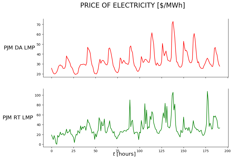
3 DATA PREPARATION
The most important aspect of data preparation will be to create an empirical distribution rather than to try and fit the data to a parametric distribution. This involves the computation of a cumulative distribution from the data. We first sort the prices from smallest to largest. Let this ordered sequence be represented by \(\tilde{p}_t\) where \(\tilde{p}_{t-1} \le \tilde{p}_t\). Also, let \(T\) be the number of time periods. The percentage of time periods with a price less than \(\tilde{p}_t\) is then \(t/T\). The empirical cumulative distribution is given by \[ F_P(\tilde{p}_t) = \frac{t}{T} \]
# hide
df_hist_price = pd.DataFrame({'hist_price': exogParams['hist_price']});
print(df_hist_price.shape)
# print(df_hist_price)
# df_hist_price.plot('hist_price');
# df_hist_price.plot();
(192, 1)df_price_changes_sorted = pd.DataFrame({'price_changes_sorted': exogParams['price_changes_sorted']});
print(df_price_changes_sorted.shape)
# print(df_price_changes_sorted)
df_price_changes_sorted.plot(figsize=(10,5));(191, 1)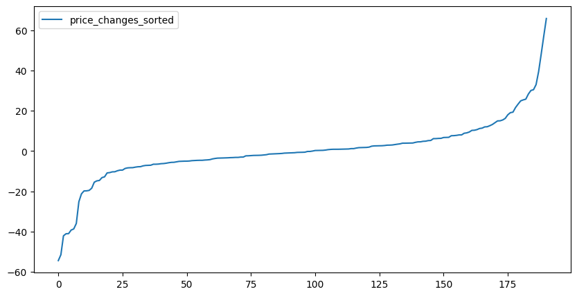
df_discrete_price_change_list = pd.DataFrame(
    {'discrete_price_change_list': exogParams['discrete_price_change_list']})
print(df_discrete_price_change_list.shape)
# print(df_discrete_price_change_list)
df_discrete_price_change_list.plot(figsize=(10,5));
(50, 1)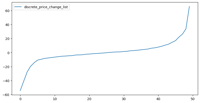
df_discrete_price_change_cdf = pd.DataFrame(
    {'discrete_price_change_cdf': exogParams['discrete_price_change_cdf']})
print(df_discrete_price_change_cdf.shape)
# print(df_discrete_price_change_cdf)
# df_discrete_price_change_cdf.plot(figsize=(10,5));
(50, 1)4 MODELING
4.1 Narrative
There has been an interest making use of batteries to exploit electricity price spikes. Power is bought when the price is low and power is sold when the price is high. This is known as battery arbitrage.
This project hightlights some interesting aspects of this kind of problem. Among these are:
- Electricity prices on the grid can be very volatile (varies between about $20/MWh to about $1,000/MWh or even $10,000/MWh for brief periods)
- Prices change every 5 minutes
- We assume that we can observe the price and then decide if we want to buy or sell
- We can only buy or sell for an entire 5-minute interval at a maximum rate of 0.01 MW
- Wind energy can be forecasted but not very well. Rolling forecasts can be used.
- Energy demand is variable but quite predictable. It depends on:
- temperature (primarily)
- humidity (less)
- Energy may be bought from or sold to the grid at current grid prices.
- There is a 5% to 10% loss when converting power from AC (grid) to DC (to store in battery).
4.2 Core Elements
This section attempts to answer three important questions: - What metrics are we going to track? - What decisions do we intend to make? - What are the sources of uncertainty?
For this problem, the only metric we are interested in is the amount of profit we make after each decision window. A single type of decision needs to be made at the start of each window - how much energy to buy or sell. The only source of uncertainty is the price of energy.
4.3 Mathematical Model | SUM Design
A Python class is used to implement the model for the SUM (System Under Management):
class EnergyStorageModel():
        def __init__(
        self, SVarNames, xVarNames, S_0, params, exogParams, possibleDecisions,
        W_fn=None, S__M_fn=None, C_fn=None):
        ...
        ...
4.3.1 State variables
The state variables represent what we need to know.
- \(R_t\)
- amount of energy stored in the battery at time \(t\)
- measured in kWh or MWh
- \(p_t\)
- price of energy on the grid
The state is:
\(S_t = (R_t,p_t)\)
The state variables are represented by the following variables in the EnergyStorageModel class:
        self.SVarNames = SVarNames
        self.State = namedtuple('State', SVarNames) # 'class'
        self.S_t = self.build_state(self.S_0) # 'instance'
where
SVarNames = ['R_t', 'p_t']4.3.2 Decision variables
The decision variables represent what we control.
- \(x_t\)
- amount of energy bought from (\(x_t>0\)) or sold to (\(x_t<0\)) the grid
- Losses
- When energy is transferred to or from the battery a loss is incurred
- Assume the loss into the battery is the same as the loss out of the battery
- \(\eta\) is the fraction of the energy retained
- \(1 - \eta\) is the loss
- Constraints
- buy from grid \((x_t>0)\):
- \(x_t \le \frac{1}{\eta}(R^{max} - R_t)\)
- sell to grid \((x_t<0)\):
- \(-x_t \le R_t\), which comes to
- \(x_t \ge -R_t\)
- buy from grid \((x_t>0)\):
- Decisions are made with a policy (TBD below):
- \(X^{\pi}(S_t)\)
The decision variables are represented by the following variables in the EnergyStorageModel class:
self.Decision = namedtuple('Decision', xVarNames) # 'class'where
xVarNames = ['x_t_EL', 'x_t_EB', 'x_t_GL', 'x_t_GB', 'x_t_BL']NOTE: For now, we will only use a single decision variable, ‘x_t_GB’. In the future the complete list will be used. In this notebook we will start to move away from the 1-hot representation.
4.3.3 Exogenous information variables
The exogenous information variables represent what we did not know (when we made a decision). These are the variables that we cannot control directly. The information in these variables become available after we make the decision \(x_t\).
When we assume that the price in each time period is revealed, without any model to predict the price based on past prices, we have:
\[ W_{t+1} = p_{t+1} \]
Alternatively, when we assume that we observe the change in price \(\hat{p}=p_t-p_{t-1}\), we have:
\[ W_{t+1} = \hat{p}_{t+1} \]
The exogenous information have been preprocessed and is captured in:
exogParams['hist_price']exogParams['price_changes_sorted']exogParams['discrete_price_change_list']exogParams['discrete_price_change_cdf']
The latest exogenous information can be accesses by calling the following method from class EnergyStorageModel():
def W_fn(self, t):
  W_tt1 = self.exogParams['hist_price'][t]
  return W_tt1
4.3.4 Transition function
The transition function describe how the state variables evolve over time. Because we currently have two state variables in the state, \(S_t=(R_t,p_t)\), we have the equations:
\[ \begin{aligned} R_{t+1} &= R_t + \eta x_t \\ p_{t+1} &= p_t + \hat{p}_{t+1} \end{aligned} \]
Collectively, they represent the general transition function:
\[ S_{t+1} = S^M(S_t,X^{\pi}(S_t)) \]
The transition function is implemented by the following method in class EnergyStorageModel():
def S__M_fn(self, t, x_t): #.
    p_tt1 = self.W_fn(t)
    R_tt1 = self.S_t.R_t + x_t.x_t_GB

    if len(self.SVarNames) == 2:
        S_tt1 = self.build_state({'R_t': R_tt1, 'p_t': p_tt1})
    elif len(self.SVarNames) == 3:
        S_tt1 = self.build_state({'R_t': R_tt1, 'p_t': p_tt1, 'p_t_1': self.S_t.p_t})
    return S_tt1
4.3.5 Objective function
The objective function captures the performance metrics of the solution to the problem. It is given by:
\[ \max_{\pi} \mathbb{E} \sum_{t=0}^T C(S_t,x_t) \]
where \[ C(S_t,x_t) = -p_tx_t \]
The contribution (reward) function is implemented by the following method in class EnergyStorageModel():
def C_fn(self, x_t):
    C_t = self.S_t.p_t*( -self.initArgs['eta']*x_t.x_t_GB )#. C(S_t, x_t, W_t+1); x_t_GB>0 for buy, <0 for sell
    return C_t
4.3.6 Implementation of SUM Model
Here is the complete implementation of the EnergyStorageModel class:
class EnergyStorageModel():
    def __init__(
        self, SVarNames, xVarNames, S_0, params, exogParams, possibleDecisions,
        W_fn=None, S__M_fn=None, C_fn=None):
        self.initArgs = params
        self.prng = np.random.RandomState(params['seed'])
        self.exogParams = exogParams
        self.S_0 = S_0
        self.SVarNames = SVarNames
        self.xVarNames = xVarNames
        self.possibleDecisions = possibleDecisions
        self.State = namedtuple('State', SVarNames) # 'class'
        self.S_t = self.build_state(self.S_0) # 'instance'
        self.Decision = namedtuple('Decision', xVarNames) # 'class'
        self.cumC = 0.0 #. cumulative reward; use F or cumF for final (i.e. no cumulative) reward
        # self.states = [self.S_t] # keep a list of states visited

    def reset(self):
        self.cumC = 0.0
        self.S_t = self.build_state(self.S_0)
        # self.states = [self.S_t]

    def build_state(self, info):
        return self.State(*[info[sn] for sn in self.SVarNames])

    def build_decision(self, info):
        return self.Decision(*[info[xn] for xn in self.xVarNames])

    def W_fn(self, t):
        W_tt1 = self.exogParams['hist_price'][t]
        return W_tt1

    def S__M_fn(self, t, x_t): #.
        p_tt1 = self.W_fn(t)
        R_tt1 = self.S_t.R_t + x_t.x_t_GB

        if len(self.SVarNames) == 2:
            S_tt1 = self.build_state({'R_t': R_tt1, 'p_t': p_tt1})
        elif len(self.SVarNames) == 3:
            S_tt1 = self.build_state({'R_t': R_tt1, 'p_t': p_tt1, 'p_t_1': self.S_t.p_t})
        return S_tt1

    def C_fn(self, x_t):
        C_t = self.S_t.p_t*( -self.initArgs['eta']*x_t.x_t_GB )#. C(S_t, x_t, W_t+1); x_t_GB>0 for buy, <0 for sell
        return C_t

    def step(self, t, x_t):
        self.cumC += self.C_fn(x_t)
        self.S_t = self.S__M_fn(t, x_t)
        return (self.S_t, self.cumC, x_t) #. for plotting
4.4 Uncertainty Model
As mentioned above in section 3, we make use of an empirical distribution rather than to try and fit the data to a parametric distribution. This involves the computation of a cumulative distribution from the data. We first sort the prices from smallest to largest. Let this ordered sequence be represented by \(\tilde{p}_t\) where \(\tilde{p}_{t-1} \le \tilde{p}_t\). Also, let \(T\) be the number of time periods. The percentage of time periods with a price less than \(\tilde{p}_t\) is then \(t/T\). The empirical cumulative distribution is given by \[ F_P(\tilde{p}_t) = \frac{t}{T} \]
4.5 Policy Design
There are two main meta-classes of policy design. Each of these has two subclasses: - Policy Search - Policy Function Approximations (PFAs) - Cost Function Approximations (CFAs) - Lookahead - Value Function Approximations (VFAs) - Direct Lookaheads (DLAs)
In this project we will use: - A simple buy low, sell high parameterized policy (from the PFA class)
The buy low, sell high policy is implemented by the following method in class EnergyStoragePolicy():
def X__BuyLowSellHigh(self, t, S_t, theta, T): # SDAM-9.4.1
    info = {
        'x_t_EL': 0, #Wind to Load ('EC': Wind to Consumer)
        'x_t_EB': 0, #Wind to Battery ('WS': Wind to Storage)
        'x_t_GL': 0, #Grid to Load ('GC': Grid to Consumer)
        'x_t_GB': 0, #Grid to Battery ('GS': Grid to Storage); can be negative to reverse flow (sell back to Grid)
        'x_t_BL': 0, #Battery to Load ('SC': Storage to Consumer)
    }
    if t >= T:
        print(f"ERROR: t={t} should not reach or exceed the max steps ({T})")
        return self.model.build_decision(info)
    if t == T - 1: #Last time period - sell
        info['x_t_GB'] = -S_t.R_t #sell the whole inventory
        # print(f'last t for this sample-path: selling all ...')
    else:
        # (SDAM-eq9.11): X^lohi(S_t|theta)
        theta__buy = theta[0] # theta__buy
        theta__sell = theta[1] # theta__sell
        if S_t.p_t <= theta__buy: # BUY if p_t <= theta__buy
            info['x_t_GB'] = (self.model.initArgs['R__max'] - S_t.R_t)/self.model.initArgs['eta']
        elif S_t.p_t >= theta__sell: # SELL if p_t >= theta__sell
            info['x_t_GB'] = -S_t.R_t #sell the whole inventory
        else: # HOLD if theta__buy < p_t < theta__sell
            info['x_t_GB'] = 0
    return self.model.build_decision(info)
4.5.1 Implementation of Policy Design
The EnergyStoragePolicy() class implements the policy design.
import random
class EnergyStoragePolicy():
    def __init__(self, model, piNames):
        self.model = model
        self.piNames = piNames
        self.Policy = namedtuple('Policy', piNames)

    def X__BuyLowSellHigh(self, t, S_t, theta, T): # SDAM-9.4.1
        info = {
            'x_t_EL': 0, #Wind to Load ('EC': Wind to Consumer)
            'x_t_EB': 0, #Wind to Battery ('WS': Wind to Storage)
            'x_t_GL': 0, #Grid to Load ('GC': Grid to Consumer)
            'x_t_GB': 0, #Grid to Battery ('GS': Grid to Storage); can be negative to reverse flow (sell back to Grid)
            'x_t_BL': 0, #Battery to Load ('SC': Storage to Consumer)
        }
        if t >= T:
            print(f"ERROR: t={t} should not reach or exceed the max steps ({T})")
            return self.model.build_decision(info)
        if t == T - 1: #Last time period - sell
            info['x_t_GB'] = -S_t.R_t #sell the whole inventory
            # print(f'last t for this sample-path: selling all ...')
        else:
            # (SDAM-eq9.11): X^lohi(S_t|theta)
            theta__buy = theta[0] # theta__buy
            theta__sell = theta[1] # theta__sell
            if S_t.p_t <= theta__buy: # BUY if p_t <= theta__buy
                info['x_t_GB'] = (self.model.initArgs['R__max'] - S_t.R_t)/self.model.initArgs['eta']
            elif S_t.p_t >= theta__sell: # SELL if p_t >= theta__sell
                info['x_t_GB'] = -S_t.R_t #sell the whole inventory
            else: # HOLD if theta__buy < p_t < theta__sell
                info['x_t_GB'] = 0
        return self.model.build_decision(info)

    def run_policy(self, piInfo, piName, params):
        model_copy = copy(self.model)
        T = params['T']
        # nTrades = {'buy': 0, 'sell': 0, 'hold': 0}
        # nTrades = {'x_t_buy': 0, 'x_t_sell': 0, 'x_t_hold': 0}
        buyList = []
        sellList = []
        for t in range(T):
            x_t = getattr(self, piName)(t, model_copy.S_t, piInfo, T)
            # nTrades['x_t_buy'] += x_t.x_t_buy; #print(f'!!!!! {x_t.buy=}')
            # nTrades['x_t_sell'] += x_t.x_t_sell; #print(f'!!!!! {x_t.sell=}')
            # nTrades['x_t_hold'] += model_copy.S_t.R_t#.
            # if x_t.x_t_buy > 0:
            if x_t.x_t_GB > 0:
                buyList.append((t, model_copy.S_t.R_t, model_copy.S_t.p_t, x_t.x_t_GB, params['R__max']))
            elif x_t.x_t_GB < 0:
                sellList.append((t, model_copy.S_t.R_t, model_copy.S_t.p_t, x_t.x_t_GB, params['R__max']))
            _, _, _ = model_copy.step(t, x_t) # step the model forward one iteration
        cumC = model_copy.cumC #.
        # print(f"Energy traded - Sell: {nTrades['x_t_sell']:.2f} - Buy: {nTrades['x_t_buy']:.2f} - Hold % : {nTrades['x_t_hold']/model_copy.init_args['T']:.2f}") #.
        # print(f"Energy traded - Buy: {nTrades['x_t_buy']:.2f} - Hold: {nTrades['x_t_hold']:.2f} - Sell: {nTrades['x_t_sell']:.2f}")
        # print("Buy times and prices ")
        # for i in range(len(buy_list)):
        #     print(f"t = {buy_list[i][0]:.2f} and price = {buy_list[i][1]:.2f}") #.
        # print("Sell times and prices ")
        # for i in range(len(sell_list)):
        #     print(f"t = {sell_list[i][0]:.2f} and price = {sell_list[i][1]:.2f}") #.
        return cumC

    def run_policy_sample_paths(self, theta, piName, params):
        FhatIomega__lI = []
        for l in range(1, params['L'] + 1):
            model_copy = copy(self.model)
            record_l = [piName, theta, l]
            T = params['T']
            # nTrades = {'x_t_buy': 0, 'x_t_sell': 0, 'x_t_hold': 0}
            buyList = []
            sellList = []
            for t in range(T):
                x_t = getattr(self, piName)(t, model_copy.S_t, theta, params['T'])
                # nTrades['x_t_buy'] += x_t.x_t_buy; #print(f'!!!!! {x_t.buy=}')
                # nTrades['x_t_sell'] += x_t.x_t_sell; #print(f'!!!!! {x_t.sell=}')
                # nTrades['x_t_hold'] += model_copy.S_t.R_t
                # if x_t.x_t_buy > 0:
                if x_t.x_t_GB > 0:
                    buyList.append((t, model_copy.S_t.R_t, model_copy.S_t.p_t, x_t.x_t_GB, params['R__max']))
                elif x_t.x_t_GB < 0:
                    sellList.append((t, model_copy.S_t.R_t, model_copy.S_t.p_t, x_t.x_t_GB, params['R__max']))
                _, _, _ = model_copy.step(t, x_t)
            FhatIomega__lI.append(model_copy.cumC) #. just above (SDAM-eq2.9) #. Fhat for this sample-path is in model_copy.cumC
            # print(f"Inventory traded - Buy: {nTrades['x_t_buy']:.2f} - Hold: {nTrades['x_t_hold']:.2f} - Sell: {nTrades['x_t_sell']:.2f}")
            # print("Buy times ")
            # for i in range(len(buy_list)):
            #     print(f"t={buy_list[i][0]}, R_t={buy_list[i][1]:.2f}, D_t={buy_list[i][2]:.2f}, x_t.x_t_buy={buy_list[i][3]:.2f}, R__max={buy_list[i][4]:.2f}")
            # print("Sell times ")
            # for i in range(len(sell_list)):
            #     print(f"t={sell_list[i][0]}, R_t={sell_list[i][1]:.2f}, D_t={sell_list[i][2]:.2f}, x_t.x_t_sell={sell_list[i][3]:.2f}, R__max={buy_list[i][4]:.2f}")
            # return cumC
        # end L
        return FhatIomega__lI

    def perform_grid_search(self, params, thetaValues):
        tS = time.time()
        cumCI_theta_I = {}
        bestTheta = None
        for theta in thetaValues:
            #print("Starting theta {}".format(theta))
            if theta[0] >= theta[1]:
                cumCI_theta_I[theta] = 0
            else:
                # print(f'\n=== {theta=} ===')
                cumC = self.run_policy(theta, "X__BuyLowSellHigh", params)
                cumCI_theta_I[theta] = cumC
                best_theta = max(cumCI_theta_I, key=cumCI_theta_I.get)
                # print(f"Finishing theta {theta} with cumC {cumC:.2f}. Best theta so far {best_theta}. Best cumC {cumCI_theta_I[best_theta]:.2f}")
        print(f"Finishing GridSearch in {time.time() - tS:.2f} secs")
        print(f"Best theta: {best_theta}. Best cumC: {cumCI_theta_I[best_theta]:.2f}")
        return cumCI_theta_I

    def perform_grid_search_sample_paths(self, params, thetaValues):
        tS = time.time()
        Fhat_mean = None
        Fhat_var = None
        Fhat__meanI_th_I = {}
        Fhat__stdvI_th_I = {}
        Fhat_mean = None
        for theta in thetaValues:
            if theta[0] >= theta[1]:
                Fhat__meanI_th_I[theta] = 0
                # pass
            else:
                # print(f'\n=== {theta=} ===')
                FhatIomega__lI = self.run_policy_sample_paths(theta, "X__BuyLowSellHigh", params)
                Fhat_mean = np.array(FhatIomega__lI).mean() #. (SDAM-eq2.9); call Fbar in future
                Fhat_var = np.sum(np.square(np.array(FhatIomega__lI) - Fhat_mean))/(params['L'] - 1)
                Fhat__meanI_th_I[theta] = Fhat_mean
                Fhat__stdvI_th_I[theta]= np.sqrt(Fhat_var/params['L'])
                best_theta = max(Fhat__meanI_th_I, key=Fhat__meanI_th_I.get)
                # print(f"Finishing theta {theta} with cumC {Fhat__meanI_th_I[best_theta]:.2f}. Best theta so far {best_theta}. Best cumC {Fhat__meanI_th_I[best_theta]:.2f}")
        print(f"Finishing GridSearch in {time.time() - tS:.2f} secs")
        print(f"Best theta: {best_theta}. Best cumC {Fhat__meanI_th_I[best_theta]:.2f}")
        # return cumCI_theta_I
        return Fhat__meanI_th_I, Fhat__stdvI_th_I

    def grid_search_theta_values(self, params):
        """
        this function gives a list of theta values needed to run a full grid search
        """
        theta_buy_values = np.arange(params['theta_buy_min'], params['theta_buy_max'], params['theta_inc'])
        theta_sell_values = np.arange(params['theta_sell_min'], params['theta_sell_max'], params['theta_inc'])

        theta_values = [(x, y) for x in theta_buy_values for y in theta_sell_values]
        return theta_values, theta_buy_values, theta_sell_values

    def plot_heat_map(self, contribution_dict, theta_buy_values, theta_sell_values):
        contribution_values = [contribution_dict[(theta_buy,theta_sell)]  for theta_sell in theta_sell_values for theta_buy in theta_buy_values]
        contributions = np.array(contribution_values)
        increment_count = len(theta_buy_values)
        contributions = np.reshape(contributions, (-1, increment_count))

        fig, ax = plt.subplots()
        im = ax.imshow(contributions, cmap='hot',origin='lower',aspect='auto')
        # create colorbar
        cbar = ax.figure.colorbar(im, ax=ax)
        # cbar.ax.set_ylabel(cbarlabel, rotation=-90, va="bottom")
        # we want to show all ticks...
        ax.set_xticks(np.arange(0,len(theta_buy_values),5))
        ax.set_yticks(np.arange(0,len(theta_sell_values),5))
        # ... and label them with the respective list entries
        ax.set_xticklabels(theta_buy_values[::5])
        ax.set_yticklabels(theta_sell_values[::5])
        # rotate the tick labels and set their alignment.
        #plt.setp(ax.get_xticklabels(), rotation=45, ha="right",rotation_mode="anchor")
        ax.set_title("Heatmap of contribution values across different values of theta")

        ax.set_ylabel('Theta sell high values')
        ax.set_xlabel('Theta buy low values')

        #fig.tight_layout()
        plt.show()
        return True
4.6 Evaluating Policies
4.6.1 Training/Tuning
# UPDATE PARAMETERS
params.update({'Algorithm': 'GridSearch'}); pprint(f'{params=}')
params.update({'R__max': 1})
params.update({'R_0': 0})
params.update({'L': 500}) #add sample-paths
params.update({'T': 100}) #optimal theta not consistent, so raise T
params
("params={'Algorithm': 'GridSearch', 'T': 192, 'eta': 0.9, 'R__max': 1, 'R_0': "
"1, 'seed': 189654913, 'theta_sell_min': 10, 'theta_sell_max': 100, "
"'theta_buy_min': 10, 'theta_buy_max': 100, 'theta_inc': 1, "
"'nPriceChangeInc': 50, 'priceDiscSet': '1, 0.5', 'run3D': False, "
"'price_disc_list': [1.0, 0.5]}"){'Algorithm': 'GridSearch',
'T': 100,
'eta': 0.9,
'R__max': 1,
'R_0': 0,
'seed': 189654913,
'theta_sell_min': 10,
'theta_sell_max': 100,
'theta_buy_min': 10,
'theta_buy_max': 100,
'theta_inc': 1,
'nPriceChangeInc': 50,
'priceDiscSet': '1, 0.5',
'run3D': False,
'price_disc_list': [1.0, 0.5],
'L': 500}# create a model and a policy
piNames = ['X__BuyLowSellHigh']
SVarNames = ['R_t', 'p_t']
initialState = {
'R_t': params['R_0'],
'p_t': exogParams['hist_price'][0],
}
xVarNames = ['x_t_EL', 'x_t_EB', 'x_t_GL', 'x_t_GB', 'x_t_BL']
possibleDecisions = None
M = EnergyStorageModel(
SVarNames,
xVarNames,
initialState,
params,
exogParams,
possibleDecisions
)
P = EnergyStoragePolicy(M, piNames)%%time
##########################################################################
#GridSearch #. SDAM-9.4.1
if params['Algorithm'] == 'GridSearch':
# obtain the theta values to carry out a full grid search
grid_search_theta_values = P.grid_search_theta_values(params)
# print(grid_search_theta_values)
# use those theta values to calculate corresponding contribution values
cumCI_theta_I = \
P.perform_grid_search(params, grid_search_theta_values[0])
P.plot_heat_map(
cumCI_theta_I,
grid_search_theta_values[1],
grid_search_theta_values[2])
#
#
# OR
#
#
# Fhat__meanI_th_I, Fhat__stdvI_th_I = \
# P.perform_grid_search_sample_paths(params, grid_search_theta_values[0])
# P.plot_heat_map(
# Fhat__meanI_th_I,
# grid_search_theta_values[1],
# grid_search_theta_values[2])
##################################################################################Finishing GridSearch in 3.52 secs
Best theta: (12, 38). Best cumC: 160.09
CPU times: user 4.01 s, sys: 111 ms, total: 4.13 s
Wall time: 4.05 s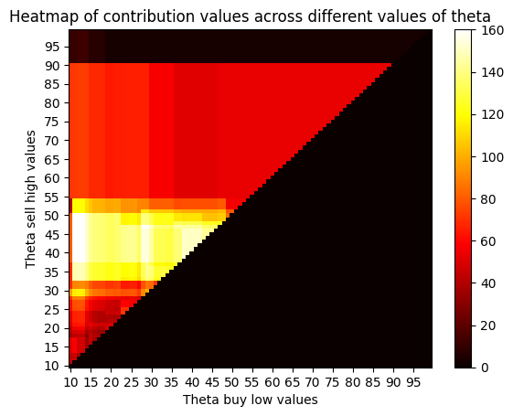
4.6.2 Evaluation
params['R_0']0# create a model and a policy
piNames = ['X__BuyLowSellHigh']
SNames = ['R_t', 'p_t']
initialState = {
# 'R_t': params['R_0'],
'R_t': 1,
'p_t': exogParams['hist_price'][0],
}
xVarNames = ['x_t_EL', 'x_t_EB', 'x_t_GL', 'x_t_GB', 'x_t_BL']
possibleDecisions = M.possibleDecisions
M_evalu = EnergyStorageModel(
SVarNames,
xVarNames,
initialState,
params,
exogParams,
possibleDecisions
)
P_evalu = EnergyStoragePolicy(M_evalu, piNames)
params{'Algorithm': 'GridSearch',
'T': 100,
'eta': 0.9,
'R__max': 1,
'R_0': 0,
'seed': 189654913,
'theta_sell_min': 10,
'theta_sell_max': 100,
'theta_buy_min': 10,
'theta_buy_max': 100,
'theta_inc': 1,
'nPriceChangeInc': 50,
'priceDiscSet': '1, 0.5',
'run3D': False,
'price_disc_list': [1.0, 0.5],
'L': 500}def run_policy_evalu(piInfo_evalu, piName_evalu, stop_time_evalu):
model_copy = copy(M_evalu)
buyList = []
sellList = []
record = [] #.
for t in range(stop_time_evalu):
x_t = getattr(P_evalu, piName_evalu)(t, model_copy.S_t, piInfo_evalu, stop_time_evalu)
if x_t.x_t_GB > 0:
buyList.append((t, model_copy.S_t.p_t))
elif x_t.x_t_GB < 0:
sellList.append((t, model_copy.S_t.p_t))
res = model_copy.step(t, x_t) # step the model forward one iteration
# print(f'{res=}')
record.append([res[0].R_t, res[0].p_t, res[1], res[2].x_t_EL, res[2].x_t_EB, res[2].x_t_GL, res[2].x_t_GB, res[2].x_t_BL])
cumC = model_copy.cumC
return cumC, record# EVALUATION
piName_evalu = 'X__BuyLowSellHigh'
stop_time_evalu = 1804.6.2.1 Optimal policy
piName_evalu'X__BuyLowSellHigh'theta_evalu = (12, 38)
cumC, record = run_policy_evalu(theta_evalu, piName_evalu, stop_time_evalu)
labels = ["R_t", "p_t", "cumC", 'x_t_EL', 'x_t_EB', 'x_t_GL', 'x_t_GB', 'x_t_BL']
print(f'{theta_evalu=}')
df = pd.DataFrame.from_records(data=record, columns=labels); df[:20]theta_evalu=(12, 38)| R_t | p_t | cumC | x_t_EL | x_t_EB | x_t_GL | x_t_GB | x_t_BL | |
|---|---|---|---|---|---|---|---|---|
| 0 | 1.0000 | 18.9100 | 0.0000 | 0 | 0 | 0 | 0.0000 | 0 |
| 1 | 1.0000 | 14.2700 | 0.0000 | 0 | 0 | 0 | 0.0000 | 0 |
| 2 | 1.0000 | 9.6700 | 0.0000 | 0 | 0 | 0 | 0.0000 | 0 |
| 3 | 1.0000 | 17.6800 | 0.0000 | 0 | 0 | 0 | 0.0000 | 0 |
| 4 | 1.0000 | 11.8800 | 0.0000 | 0 | 0 | 0 | 0.0000 | 0 |
| 5 | 1.0000 | 2.0800 | 0.0000 | 0 | 0 | 0 | 0.0000 | 0 |
| 6 | 1.0000 | 0.0000 | 0.0000 | 0 | 0 | 0 | 0.0000 | 0 |
| 7 | 1.0000 | 18.0000 | 0.0000 | 0 | 0 | 0 | 0.0000 | 0 |
| 8 | 1.0000 | 14.4800 | 0.0000 | 0 | 0 | 0 | 0.0000 | 0 |
| 9 | 1.0000 | 17.8800 | 0.0000 | 0 | 0 | 0 | 0.0000 | 0 |
| 10 | 1.0000 | 24.6400 | 0.0000 | 0 | 0 | 0 | 0.0000 | 0 |
| 11 | 1.0000 | 19.5700 | 0.0000 | 0 | 0 | 0 | 0.0000 | 0 |
| 12 | 1.0000 | 20.2600 | 0.0000 | 0 | 0 | 0 | 0.0000 | 0 |
| 13 | 1.0000 | 22.2100 | 0.0000 | 0 | 0 | 0 | 0.0000 | 0 |
| 14 | 1.0000 | 18.5200 | 0.0000 | 0 | 0 | 0 | 0.0000 | 0 |
| 15 | 1.0000 | 18.7800 | 0.0000 | 0 | 0 | 0 | 0.0000 | 0 |
| 16 | 1.0000 | 23.0900 | 0.0000 | 0 | 0 | 0 | 0.0000 | 0 |
| 17 | 1.0000 | 30.6900 | 0.0000 | 0 | 0 | 0 | 0.0000 | 0 |
| 18 | 1.0000 | 22.8800 | 0.0000 | 0 | 0 | 0 | 0.0000 | 0 |
| 19 | 1.0000 | 24.6000 | 0.0000 | 0 | 0 | 0 | 0.0000 | 0 |
df.tail()| R_t | p_t | cumC | x_t_EL | x_t_EB | x_t_GL | x_t_GB | x_t_BL | |
|---|---|---|---|---|---|---|---|---|
| 175 | 0.0000 | 30.3400 | 207.3490 | 0 | 0 | 0 | 0.0000 | 0 |
| 176 | 0.0000 | 41.5300 | 207.3490 | 0 | 0 | 0 | 0.0000 | 0 |
| 177 | 0.0000 | 107.3400 | 207.3490 | 0 | 0 | 0 | -0.0000 | 0 |
| 178 | 0.0000 | 87.5700 | 207.3490 | 0 | 0 | 0 | -0.0000 | 0 |
| 179 | 0.0000 | 36.0800 | 207.3490 | 0 | 0 | 0 | -0.0000 | 0 |
4.6.2.2 Non-optimal policy
theta_evalu_non=(30, 95)
cumC, record = run_policy_evalu(theta_evalu_non, piName_evalu, stop_time_evalu)
labels = ["R_t", "p_t", "cumC", 'x_t_EL', 'x_t_EB', 'x_t_GL', 'x_t_GB', 'x_t_BL']
print(f'{theta_evalu_non=}')
df_non = pd.DataFrame.from_records(data=record, columns=labels); df[:20]
theta_evalu_non=(30, 95)| R_t | p_t | cumC | x_t_EL | x_t_EB | x_t_GL | x_t_GB | x_t_BL | |
|---|---|---|---|---|---|---|---|---|
| 0 | 1.0000 | 18.9100 | 0.0000 | 0 | 0 | 0 | 0.0000 | 0 |
| 1 | 1.0000 | 14.2700 | 0.0000 | 0 | 0 | 0 | 0.0000 | 0 |
| 2 | 1.0000 | 9.6700 | 0.0000 | 0 | 0 | 0 | 0.0000 | 0 |
| 3 | 1.0000 | 17.6800 | 0.0000 | 0 | 0 | 0 | 0.0000 | 0 |
| 4 | 1.0000 | 11.8800 | 0.0000 | 0 | 0 | 0 | 0.0000 | 0 |
| 5 | 1.0000 | 2.0800 | 0.0000 | 0 | 0 | 0 | 0.0000 | 0 |
| 6 | 1.0000 | 0.0000 | 0.0000 | 0 | 0 | 0 | 0.0000 | 0 |
| 7 | 1.0000 | 18.0000 | 0.0000 | 0 | 0 | 0 | 0.0000 | 0 |
| 8 | 1.0000 | 14.4800 | 0.0000 | 0 | 0 | 0 | 0.0000 | 0 |
| 9 | 1.0000 | 17.8800 | 0.0000 | 0 | 0 | 0 | 0.0000 | 0 |
| 10 | 1.0000 | 24.6400 | 0.0000 | 0 | 0 | 0 | 0.0000 | 0 |
| 11 | 1.0000 | 19.5700 | 0.0000 | 0 | 0 | 0 | 0.0000 | 0 |
| 12 | 1.0000 | 20.2600 | 0.0000 | 0 | 0 | 0 | 0.0000 | 0 |
| 13 | 1.0000 | 22.2100 | 0.0000 | 0 | 0 | 0 | 0.0000 | 0 |
| 14 | 1.0000 | 18.5200 | 0.0000 | 0 | 0 | 0 | 0.0000 | 0 |
| 15 | 1.0000 | 18.7800 | 0.0000 | 0 | 0 | 0 | 0.0000 | 0 |
| 16 | 1.0000 | 23.0900 | 0.0000 | 0 | 0 | 0 | 0.0000 | 0 |
| 17 | 1.0000 | 30.6900 | 0.0000 | 0 | 0 | 0 | 0.0000 | 0 |
| 18 | 1.0000 | 22.8800 | 0.0000 | 0 | 0 | 0 | 0.0000 | 0 |
| 19 | 1.0000 | 24.6000 | 0.0000 | 0 | 0 | 0 | 0.0000 | 0 |
4.6.2.3 Visualization
from certifi.core import where
def plot_output(df1, df2):
n_charts = 4
ylabelsize = 16
mpl.rcParams['lines.linewidth'] = 1.2
fig, axs = plt.subplots(n_charts, sharex=True)
# fig.set_figwidth(50); fig.set_figheight(20)
fig.set_figwidth(13); fig.set_figheight(9)
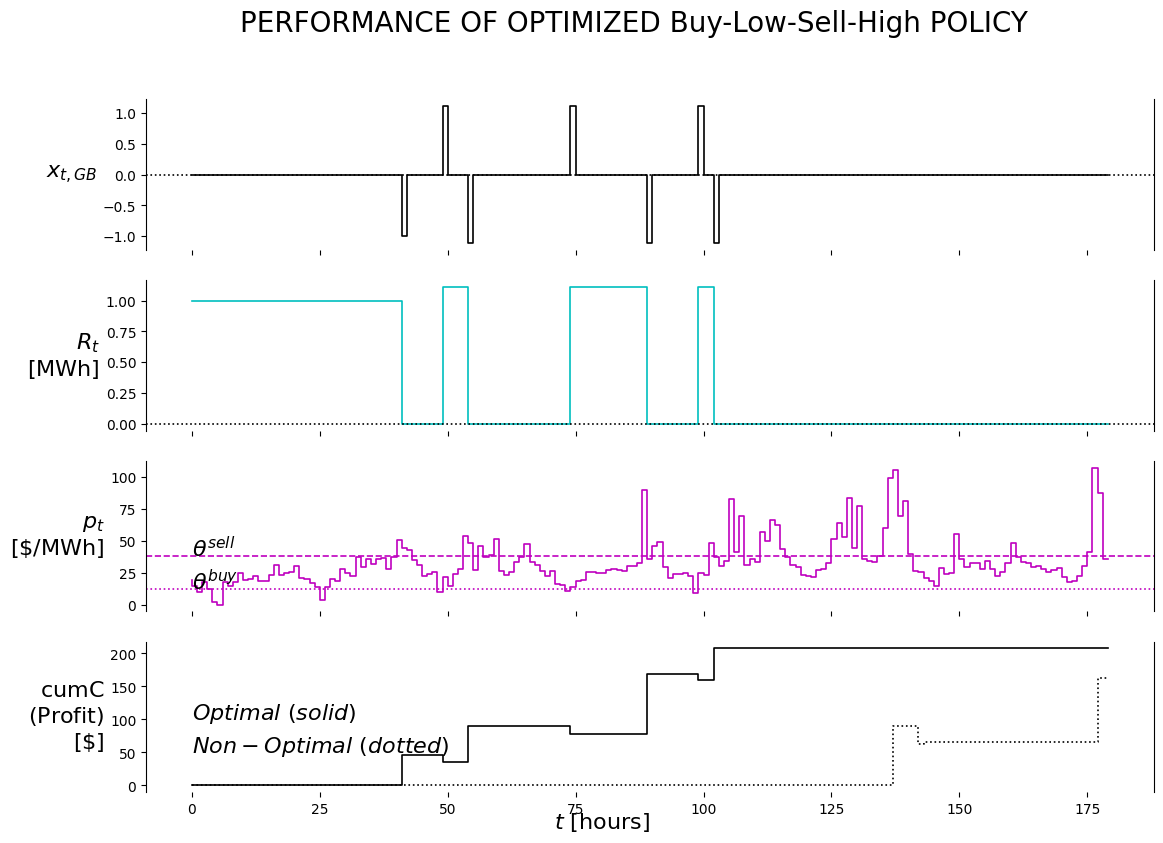
fig.suptitle('PERFORMANCE OF OPTIMIZED Buy-Low-Sell-High POLICY', fontsize=20)
i = 0 #buy/hold/sell
axs[i].set_ylim(auto=True); axs[i].spines['top'].set_visible(False); axs[i].spines['right'].set_visible(True); axs[i].spines['bottom'].set_visible(False)
axs[i].step(df1['x_t_GB'], 'k')
axs[i].axhline(y=0, color='k', linestyle=':')
axs[i].set_ylabel('$x_{t,GB}$', rotation=0, ha='right', va='center', fontweight='bold', size=ylabelsize);
i = 1 #R_t
axs[i].set_ylim(auto=True); axs[i].spines['top'].set_visible(False); axs[i].spines['right'].set_visible(True); axs[i].spines['bottom'].set_visible(False)
axs[i].step(df1['R_t'], 'c')
axs[i].axhline(y=0, color='k', linestyle=':')
axs[i].set_ylabel('$R_t$'+'\n'+'$\mathrm{[MWh]}$', rotation=0, ha='right', va='center', fontweight='bold', size=ylabelsize);
i = 2 #p_t
axs[i].set_ylim(auto=True); axs[i].spines['top'].set_visible(False); axs[i].spines['right'].set_visible(True); axs[i].spines['bottom'].set_visible(False)
axs[i].step(df1['p_t'], 'm')
axs[i].axhline(y=theta_evalu[0], color='m', linestyle=':')
axs[i].text(0, theta_evalu[0], r'$\theta^{buy}$', size=16)
axs[i].axhline(y=theta_evalu[1], color='m', linestyle='--')
axs[i].text(0, theta_evalu[1], r'$\theta^{sell}$', size=16)
axs[i].set_ylabel('$p_t$'+'\n'+'$\mathrm{[\$/MWh]}$', rotation=0, ha='right', va='center', fontweight='bold', size=ylabelsize);
i = 3 #cumC
axs[i].set_ylim(auto=True); axs[i].spines['top'].set_visible(False); axs[i].spines['right'].set_visible(True); axs[i].spines['bottom'].set_visible(False)
axs[i].step(df1['cumC'], 'k')
axs[i].step(df2['cumC'], 'k:')
axs[i].text(0, 100, r'$Optimal\ (solid)$', size=16)
axs[i].text(0, 50, r'$Non-Optimal\ (dotted)$', size=16)
axs[i].set_ylabel('$\mathrm{cumC}$'+'\n'+'$\mathrm{(Profit)}$'+'\n'+''+'$\mathrm{[\$]}$', rotation=0, ha='right', va='center', fontweight='bold', size=ylabelsize);
axs[i].set_xlabel('$t\ \mathrm{[hours]}$', rotation=0, ha='right', va='center', fontweight='bold', size=ylabelsize);
plot_output(df, df_non)